Modelling acoustic wave propagation in batteries

Acoustic methods are an increasingly attractive way to probe battery state without tearing cells apart. Changes in temperature, state of charge and mechanical condition all affect how acoustic waves travel through a cell. The challenge is not generating acoustic signals; it’s interpreting them.

During a consultancy project with Sention, we built a modelling framework designed to bridge that gap: a fast, configurable acoustic wave model of a layered battery structure that could be rerun by non-modelling specialists to match experimental data and extract effective material properties.

This post outlines the design decisions behind that framework, from the physical model through to the software architecture, and why simplicity and efficiency mattered more than dimensional fidelity.

Design goals

Usable by non-modellersExperimentalists needed to rerun simulations without touching PDE solvers or numerical settings.

Fast and configurableParameter variation across electrodes, separators and current collectors: acoustic velocity, density, impedance, attenuation.

Scalable for dataset generationNot just individual fits, but a large synthetic dataset for future machine learning models.

Physically grounded but minimalThe dominant physics of wave propagation, without unnecessary complexity.

This led directly to a 1D layered acoustic model, prioritising speed, robustness and interpretability.

Physical model: 1D layered acoustics

The battery was represented as a 1D stack of material layers: positive electrode, separator, negative electrode and current collectors. Each layer was assigned its own acoustic properties (wave speed, density, impedance), allowing discontinuities at interfaces and reflections to emerge naturally from the physics.

While clearly an approximation, the 1D assumption offered two key advantages:

It captures the dominant through-thickness wave behaviour relevant to many experimental setups.
It allows extremely fast simulation and dense parameter sweeps.

The goal was never to perfectly reproduce every experimental detail, but to build a useful inverse tool.

Numerical engine: why Clawpack?

For the underlying physics engine, we used Clawpack, a finite-volume framework designed for hyperbolic PDEs and wave propagation problems. It provides:

Robust handling of wave propagation and reflections
Clear separation between physics and numerics
Excellent performance for 1D problems
Mature, well-tested solvers

Crucially, it allowed the physics to remain explicit and inspectable, rather than hidden behind a black-box solver.

A domain-specific API for battery acoustics

To make the model usable, we built a small domain-specific API on top of Clawpack. Instead of defining grids and coefficients manually, users specify layer ordering, thicknesses, acoustic properties per layer, and source and sensor locations. Changing a material property or layer configuration became a matter of editing a few parameters, not rewriting solver code.

End-to-end architecture

To make the system easy to deploy and rerun, the full workflow was containerised and split into three components.

component	what it does
Backend	Dockerised Clawpack simulation server, exposed through a FastAPI interface for parameterised runs.
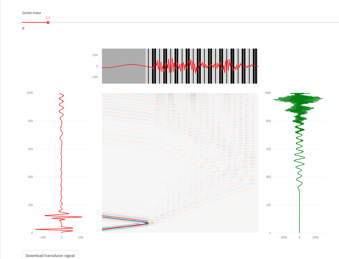
Frontend	Built in Streamlit. Interactive control of layer properties and immediate visualisation of wave propagation and received signals.
Workflow	Select layer properties and conditions, run the simulation, visualise the results, adjust parameters to match experimental data.

This setup allowed experimentalists to explore “what-if” scenarios without needing to understand the underlying PDEs.

Matching experimental data

Fix the known geometry
Vary acoustic properties with temperature and state of charge
Compare simulated and measured signals
Identify effective material parameters that best explain the data

Because simulations were fast and reproducible, it was practical to run large parameter sweeps and build intuition about sensitivity and identifiability.

Towards data-driven interpretation

The longer-term vision was to generate large synthetic datasets spanning material property variations, temperature and state of charge. These could train machine learning models to interpret acoustic signals rapidly, learning the inverse mapping that is expensive to compute directly. The framework was designed with this step in mind from day one.

The most useful model is rarely the most detailed one.

By focusing on the dominant physics, a clean abstraction layer and strong tooling around the solver, it was possible to build a framework that served both immediate experimental needs and future data-driven ambitions. If you’re interested in acoustic diagnostics, inverse problems, or building modelling tools that non-specialists can actually use, this approach scales surprisingly well.